Time-Varying Rates
Many scenarios raise the necessity of incorporating temporally changing rates in epidemiological models. For instance, when containment measures are continuously increased during the progression of an outbreak, rates such as the infection rate will decrease while a quarantine rate will increase. Other examples include seasonally changing infection rates.
Systems like this can be easily set up with epipack which will be demonstrated in the following.
Numeric Models
When defining rates, EpiModel explicitly checks each rate for a functional dependence. E.g. let's define a seasonally changing infection rate and pass it to a model
def infection_rate(t,y):
    return 2 + np.sin(t)

model = EpiModel(list('SIR'))
model.add_transmission_processes([
        ('S', 'I', infection_rate, 'I', 'I'),
    ])
Epipack automatically incorporates this function into its integration/simulation framework.
As one can see from the example, a functional rate
takes as input the current time t and
a state vector y. The state vector y (a numpy
array) will be passed to this function during
integration/simulation and contains the current
incidence for every compartment. Considering the example
above, y's first element corresponds to the S compartment,
the second element to the I compartment, and the third element
to the R compartment. This order is defined by the order
of the compartment list that was passed to EpiModel during
construction.
Tabulated Values
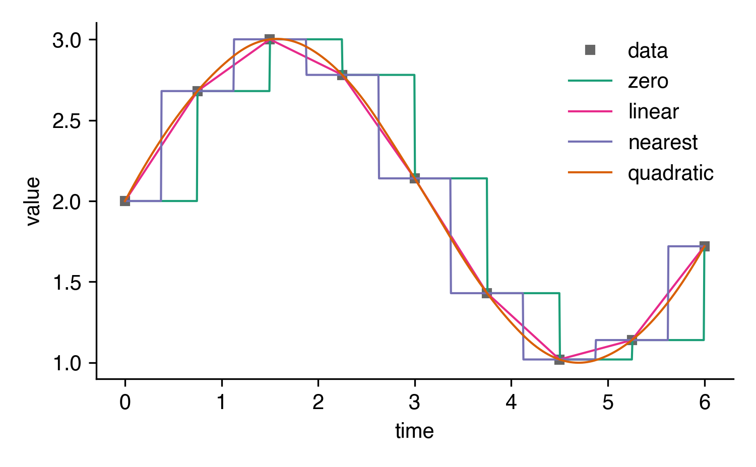
In case you're approximating continuous functions with tabulated values, e.g. when mapping an infection rate to a reduction in mobility that's only available on a weekly basis, you can use scipy's interpolation method interp1d.
Assuming we have the following tabulated data
data = np.array([
    (0.0,  2.00),
    (0.75, 2.68),
    (1.5,  3.00),
    (2.25, 2.78),
    (3.0,  2.14),
    (3.75, 1.43),
    (4.5,  1.02),
    (5.25, 1.14),
    (6.0,  1.72),
])

times, rates = data[:,0], data[:,1]
we can define our interpolated rate function using interp1d.
f = interp1d(times, rates, kind='linear')

def infection_rate(t,y):
    return f(t)
interp1d offers several different methods of interpolation
including 'zero' in case you want to use step functions.
Here's an illustration of how different kind values
shape the interpolation:
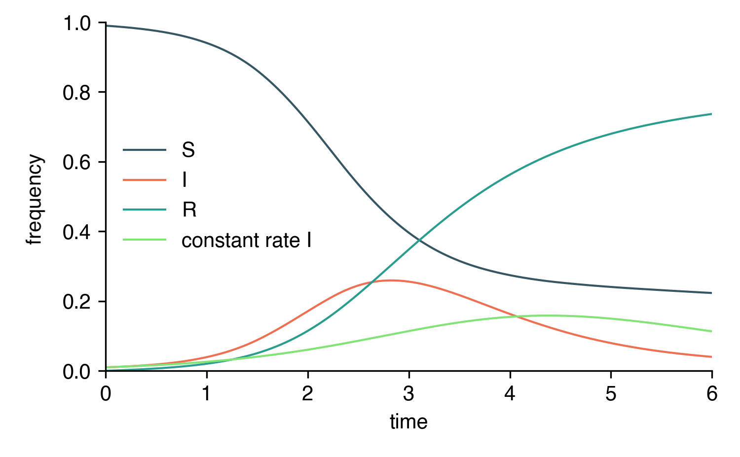
Here's a complete example script where a linearly interpolated rate is compared to a constant rate \(\eta = 2\).
from epipack import EpiModel
from scipy.interpolate import interp1d
from epipack.plottools import plot
import matplotlib.pyplot as pl
import numpy as np

data = np.array([
    (0.0,  2.00),
    (0.75, 2.68),
    (1.5,  3.00),
    (2.25, 2.78),
    (3.0,  2.14),
    (3.75, 1.43),
    (4.5,  1.02),
    (5.25, 1.14),
    (6.0,  1.72),
])

times, rates = data[:,0], data[:,1]

f = interp1d(times, rates, kind='linear', bounds_error=False)

def infection_rate(t,y):
    return f(t)

model = EpiModel(list("SIR"))
model.set_processes([
        ('S', 'I', infection_rate, 'I', 'I'),
        ('I', 1.0, 'R'),
    ])\
    .set_initial_conditions({'S':0.99,'I':0.01})\

t = np.linspace(0,6,1000)

result = model.integrate(t)
ax = plot(t,result)
ax.legend(frameon=False)

model = EpiModel(list("SIR"))
model.set_processes([
        ('S', 'I', 2.0, 'I', 'I'),
        ('I', 1.0, 'R'),
    ])\
    .set_initial_conditions({'S':0.99,'I':0.01})\

t = np.linspace(0,6,1000)

result = model.integrate(t,return_compartments='I')
ax = plot(t,result,ax=ax,curve_label_format='constant rate {}')
ax.set_ylim([0,1])
ax.legend(frameon=False)


ax.get_figure().savefig('interp_SIR_numeric.png',dpi=300)
pl.show()
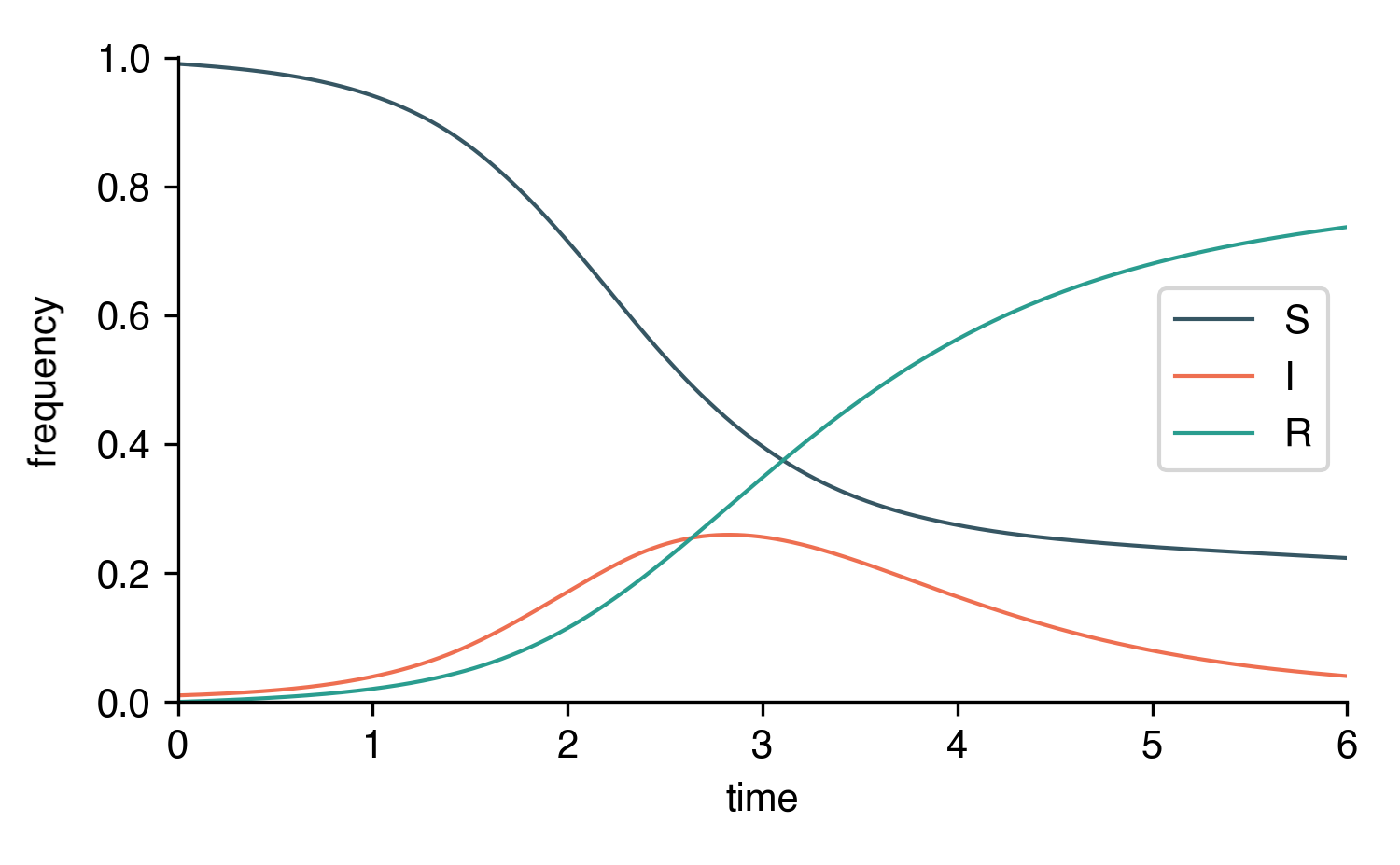
Symbolic Models
For SymbolicEpiModels, the symbol t is reserved for time.
It's simple enough to define rates like this:
import sympy

S, I, R, t, rho = sympy.symbols("S I R t rho")

model = SymbolicEpiModel([S,I,R])
model.set_processes([
        (S, I, 2+sympy.sin(t), I, I),
        (I, rho, R),
    ])
Interpolation for Tabulated Values
Similar to the framework for EpiModel, we can define symbolic interpolation functions. epipack comes with its own wrapper to define such functions.
from epipack.symbolic_epi_models import (
                get_temporal_interpolation,
                SymbolicEpiModel,
            )

data = np.array([
    (0.0,  2.00),
    (0.75, 2.68),
    (1.5,  3.00),
    (2.25, 2.78),
    (3.0,  2.14),
    (3.75, 1.43),
    (4.5,  1.02),
    (5.25, 1.14),
    (6.0,  1.72),
])

times, rates = data[:,0], data[:,1]

f = get_temporal_interpolation(times, rates, interpolation_degree=1)

S, I, R, t, rho = sympy.symbols("S I R t rho")

model = SymbolicEpiModel([S,I,R])
model.set_processes([
        (S, I, f, I, I),
        (I, rho, R),
    ])
You can use interpolation_degree = 0 to obtain step functions,
interpolation_degree = 1 to obtain linearly interpolated functions,
interpolation_degree = 2 for quadrativally interpolated functions
and so forth.
Here's a complete example script:
from epipack.symbolic_epi_models import (
                    get_temporal_interpolation,
                    SymbolicEpiModel,
                )
import sympy
from epipack.plottools import plot
from bfmplot import pl
import numpy as np

data = np.array([
    (0.0,  2.00),
    (0.75, 2.68),
    (1.5,  3.00),
    (2.25, 2.78),
    (3.0,  2.14),
    (3.75, 1.43),
    (4.5,  1.02),
    (5.25, 1.14),
    (6.0,  1.72),
])

times, rates = data[:,0], data[:,1]

f = get_temporal_interpolation(times, rates, interpolation_degree=1)

S, I, R, t, rho = sympy.symbols("S I R t rho")

model = SymbolicEpiModel([S,I,R])
model.set_processes([
        (S, I, f, I, I),
        (I, rho, R),
    ])\
    .set_initial_conditions({S:0.99,I:0.01})\
    .set_parameter_values({rho:1})

t = np.linspace(0,6,1000)

result = model.integrate(t)
ax = plot(t,result)
ax.legend()
ax.get_figure().savefig('interp_SIR_symbolic.png',dpi=300)
pl.show()