Interactive Integrations
Immediate feedback on the influence of parameter changes is a powerful mechanism to understand a system's inner workings in a fast manner. epipack therefore offers an interactive widget for Jupyter notebooks where parameter values can be changed with sliders and the influence on system trajectories is shown immediately.
Example: SIRS Model
The most efficient way to define a model for which parameter
values can be changed on the fly is by using a
epipack.symbolic_epi_models.SymbolicEpiModel (c.f. the
class' method
epipack.symbolic_epi_models.SymbolicMixin.set_parameter_values()).
Also, we need the interactive integrator class and two range classes, one for linear sliders and one for log slides.
Last but not least, tell the jupyter notebook to render matplotlib figures as widgets.
from epipack import SymbolicEpiModel
from epipack.interactive import InteractiveIntegrator, Range, LogRange
import sympy
%matplotlib widget
Now, we need to define the symbols needed for the SIRS model.
S, I, R, R0, tau, omega = sympy.symbols("S I R R_0 tau omega")
Having done that, we can define the model (with initial conditions)
I0 = 0.01
model = SymbolicEpiModel([S,I,R])\
         .set_processes([
                (S, I, R0/tau, I, I),
                (I, 1/tau, R),
                (R, omega, S),
            ])\
         .set_initial_conditions({S:1-I0, I:I0})
Here, the basic reproduction number \(R_0\), the infectious period \(\tau\), and the waning immunity rate \(\omega\) are parameters of the system. Let's say we're interested in how the system changes its behavior when \(R_0\) and \(\tau\) are varied and \(\omega\) is kept fixed.
We define:
parameters = {
    R0: LogRange(min=0.1,max=10,step_count=1000),
    tau: Range(min=0.1,max=10,value=8.0),
    omega: 1/14
}
Here, LogRange lets \(R_0\) be varied
between 0.1 and 10, based on base 10 (default base)
with 1000 steps in the exponent of the base.
Since we did not supply an initial value,
the initial value will be set to the geometric
mean of min and max, here \(R_0=1\).
Range behaves similarly, but on a linear scale,
with 100 steps (default number of steps).
If we hadn't given an initial value, it would have
chosen the mean of min and max,
here \(\tau=5.05\).
Now we can start the interactive analysis.
t = np.logspace(-3,2,1000)
InteractiveIntegrator(model, parameters, t, figsize=(4,4))
And this is the result:
More customization
Range, LogRange, and InteractiveIntegrator can be further modified.
I suggest to refer to their docstrings where these options can be further explored:
Note that InteractiveIntegrator carries the matplotlib Axes
object as an attribute. So, if you want to add more plots (e.g. data),
you can simply do that. In this case, save the integrator widget to
a variable. In this case, you need to pass this variable to jupyter
at the end of the cell.
integrator = InteractiveIntegrator(model, parameters, t, figsize=(4,4))
integrator
Now, you can access the Axes object:
integrator.ax.plot(t, data)
General interaction widget
Of course, the general interactive integrator is rather strict in the sense that only model objects can be passed to display integrated results.
Instead, one might want to display any kind of result. epipack offers the possibility
to do just that, based on the epipack.interactive.GeneralInteractiveWidget.
Here's an example to run in a Jupyter notebook. First, we have to import the relevant classes and tell Jupyter notebook that we're going to use widgets.
import epipack as epk

from epipack.interactive import GeneralInteractiveWidget, Range, LogRange
import numpy as np
%matplotlib widget
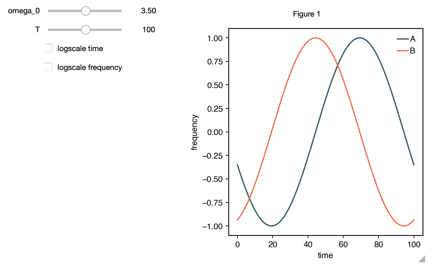
Next, we define a function that takes parameter values and returns a dictionary with time series.
t = np.linspace(0,100,1000)

def get_trig(omega_0,T):
    return {
        'A': np.sin(2*np.pi*t/T+omega_0),
        'B': np.cos(2*np.pi*t/T+omega_0),
    }

parameter_values = {
    'omega_0': Range(0,7,100),
    'T': LogRange(10,1e3,100),
}
Now, we can display the interactive widget
GeneralInteractiveWidget(get_trig,parameter_values,t,continuous_update=True)