Network/Well-Mixed Simulations
All models shown up until now ignore the explicit contact structure between individuals. Such structures can be introduced using networks where \(N\) nodes represent individuals that are connected by links.
These links represent potentially infectious contacts and can be weighted and/or directed.
Network Example
Let's assume a toy system where a central individual with id
0 is connected to two other individuals 1 and 2.
On average, node 0 spends 1/3 of their time (say, 8h a day) with individual
1 and and 2/3 of their time (16h a day) with individual 2.
The network can be defined as follows:
N = 3
edge_weight_tuples = [
    (0, 1, 1/3),
    (0, 2, 2/3),
]
directed = False
We want to investigate a scenario in which node 0 is initially
infected (in SIR dynamics)
and we're interested to find the probability that node 1 has
been infected after every individual has recovered.
First, we have to define the model
from epipack import StochasticEpiModel
S, I, R = list("SIR")

model = StochasticEpiModel(
                compartments=[S,I,R],
                N=N,
                edge_weight_tuples=edge_weight_tuples,
                directed=directed,
            )
Of course, we need to define infection and recovery processes. Infection processes are link transmission processes and are set like this:
infection_rate = 3.0
model.set_link_transmission_processes([
        ('I', 'S', infection_rate, 'I', 'I'),
    ])
Note that for link transmission processes, the
first compartment of the left hand side of
the reaction equation ('I', 'S', infection_rate, 'I', 'I')
must be an infecting compartment (the infecting compartment
of this particular reaction, not necessarily 'I') and equal to the
first compartment of the right hand side of the reaction equation.
Also, the infection_rate represents the transmission
rate per unit contact, i.e. per contact with unit weight 1.0
and will be scaled with a link's weight to form a
contact-specific infection rate.
Now, we also need to set the node transition processes.
recovery_rate = 2.0
model.set_node_transition_processes([
        ('I', recovery_rate, 'R'),
    ])
Of course, before we can do anything we have to define the initial conditions. Initial conditions are either set randomly like this:
model.set_random_initial_conditions({S: N-1, I: 1})
Yet, we said that we wanted specific initial conditions. For a StochasticEpiModel, we have to set them as a numpy array that carries the initial compartment id for every node.
initial_node_statuses = np.array([
        model.get_compartment_id(I),
        model.get_compartment_id(S),
        model.get_compartment_id(S),
    ])
model.set_node_statuses(initial_node_statuses)
Of course, nothing stops us to set this array more easily, because we know the compartment ids from the compartment list as \(C_S=0\), \(C_I=1\), and \(C_R=2\), such that
initial_node_statuses = np.zeros(N,dtype=int)
initial_node_statuses[0] = 1
model.set_node_statuses(initial_node_statuses)
Finally, we simulate this system ten thousand times
and count how often node 1 became infected.
N_meas = 10000
N_inf = 0
for meas in range(N_meas):
    model.set_node_statuses(initial_node_statuses)
    model.simulate(tmax=1e300)
    if model.node_status[1] == model.get_compartment_id(R):
        N_inf += 1

print("Node 1 has been infected in", N_inf/N_meas*100, "% of the measurements").
And this is the output:
Node 1 has been infected in 33.21 % of the measurements.
Assuming the dimension of time to be \([t] = 1/\mathrm{d}\), the link \((0,1,1/3)\) is associated with infection rate
such that a duration \(\tau_I\) until this particular infection takes place is distributed according to pdf
The infectious period of node 0 is distributed as
with \(\rho=2/\mathrm{d}\). The probability that node 1 became infected is equal to the probability that a sample \(\tau_I\) is of lower value than a sample \(\tau_R\), i.e. we need to compute
which is approximately equal to our simulation result.
We can do the same for the second link \((0, 2,2/3)\) that has link-specific infection rate \(\eta=2/\mathrm{d}\) and thus will have been infected in
of the simulations. Adjusting the code above to count the infections of node 2, we obtain
node 2 has been infected in 50.023 % of the measurements.
We can also measure the mean number of secondary infections of
node 0 (i.e. its reproduction number):
N_meas = 10000
N_inf = 0
reproduction_number = 0
for meas in range(N_meas):
    model.set_node_statuses(initial_node_statuses)
    t, result = model.simulate(tmax=1e300)
    # the number of secondary infections is given
    # by the number of recovereds at the end of the
    # simulation (minus the initial seed).
    reproduction_number += (1/N_meas) * (result['R'][-1] - 1)

print("Node 0 has infected", reproduction_number, "neighbors on average.")
We obtain:
Node 0 has infected 0.8373 neighbors on average.
We have 3 possible outcomes: zero nodes have been infected, one node has been infected, and two nodes have been infected. The probability that 0 nodes have been infected is given by the probability that node 1 has not been infected and node 2 has not been infected as
The probability that 2 nodes have been infected is given by the probability that node 1 has been infected and node 2 has been infected, which is
Because these probabilities have to sum to \(\Pi_0+\Pi_1+\Pi_2=1\) we know immediately that \(\Pi_1 = 1/2\). Nevertheless, let's write it down from first principles. The probability that 1 node has been infected is given by the probability that node 1 has been infected and node 2 has not been infected, or that node 2 has been infected and node 1 has not been infected, i.e.
Consequently, the expected reproduction number of node 0 is given as
which matches our simulation result.
And this is the entire script for copy/paste:
from epipack import StochasticEpiModel
import numpy as np

N = 3
edge_weight_tuples = [
    (0, 1, 1/3),
    (0, 2, 2/3),
]
directed = False

S, I, R = list("SIR")

model = StochasticEpiModel(
                compartments=[S,I,R],
                N=N,
                edge_weight_tuples=edge_weight_tuples,
                directed=directed,
            )

infection_rate = 3.0
model.set_link_transmission_processes([
        ('I', 'S', infection_rate, 'I', 'I'),
    ])

recovery_rate = 2.0
model.set_node_transition_processes([
        ('I', recovery_rate, 'R'),
    ])

model.set_random_initial_conditions({S: N-1, I: 1})

initial_node_statuses = np.array([
        model.get_compartment_id(I),
        model.get_compartment_id(S),
        model.get_compartment_id(S),
    ])
model.set_node_statuses(initial_node_statuses)

initial_node_statuses = np.zeros(N,dtype=int)
initial_node_statuses[0] = 1
model.set_node_statuses(initial_node_statuses)

N_meas = 10000
N_inf = 0
N_inf_node_2 = 0
for meas in range(N_meas):
    model.set_node_statuses(initial_node_statuses)
    model.simulate(tmax=1e300)
    if model.node_status[1] == model.get_compartment_id(R):
        N_inf += 1
    if model.node_status[2] == model.get_compartment_id(R):
        N_inf_node_2 += 1

print("Node 1 has been infected in", N_inf/N_meas*100, "% of the measurements.")
print("Node 2 has been infected in", N_inf_node_2/N_meas*100, "% of the measurements.")

N_meas = 10000
N_inf = 0
reproduction_number = 0
for meas in range(N_meas):
    model.set_node_statuses(initial_node_statuses)
    t, result = model.simulate(tmax=1e300)
    reproduction_number += result['R'][-1] -1

print("Node 0 has infected", reproduction_number/N_meas, "neighbors on average.")
Conditional Transmission Processes
In order to simulate processes such as contact tracing, epipack offers the possibility to define conditional transmission processes that are executed for each neighbor of a focal node when this focal node changes compartments.
Let's simulate an SAIRX system on a random graph. This system is defined as follows:
Susceptibles S can be infected both by symptomatic infectious I and asymptomatic infectious A, becoming either symptomatic infectious I or asymptomatic infectious A themselves. We also assume that infectious individuals are quarantined with a quarantine rate at which each of their contacts will be traced and isolated with probability p if they're symptomatic infectious themselves.
Processes
The node transition processes are given as
node_transition = [
    ('I', recovery_rate, 'R'),
    ('A', recovery_rate, 'R'),
    ('I', quarantine_rate, 'X'),
]
Here, we assume that both I and A individuals remain infectious for a period of mean equal length.
Also, we define transmission processes where we assume that A individuals are only half as infectious as I individuals and that 30% of all infections result in an A individual.
link_transmission = [
    ('I', 'S', infection_rate*0.7, 'I', 'I'),
    ('I', 'S', infection_rate*0.3, 'I', 'A'),
    ('A', 'S', 0.5*infection_rate*0.7, 'I', 'I'),
    ('A', 'S', 0.5*infection_rate*0.3, 'I', 'A'),
]
Now, we also said that with probability p, neighbors of quarantined individuals shall be isolated, too, if they're infectious. Therefore, we introduce the following conditional transmission process
conditional_transmission = {
    ('I', '->', 'X') : [
            ('X', 'I', p, 'X', 'X'),
        ]
}
Every neighbor of a node that transitions from I to X will transition to X themselves with probability p.
Note that generally speaking, a single one of multiple possible transmission processes could happen to each I neighbor. E.g. we could define that every I-neighbor of an X-transitioned focal node could additionally be isolated in a T (traced) compartment with probability q which could model a situation in which a fraction q of all contacts are informed of a focal node's positive infection and isolate themselves without being counted in the X compartment. In this case, the conditional transmission processes would be formulated as
conditional_transmission = {
    ('I', '->', 'X') : [
            ('X', 'I', p, 'X', 'X'),
            ('X', 'I', q, 'X', 'T'),
        ]
}
Here, every neighbor of a node that transitions from I to X will either transition to X (with probability p), transition to T (with probability q) or stay in compartment I (with probability 1-p-q). Note that the last event will always be added explicitly and automatically if not set manually.
These kinds of transmission rules have strict formatting rules that are explained in detail in section Processes.
Setup
Let's define links based on a random graph.
import networkx as nx

k0 = 50
N = int(1e4)
edges = [ (e[0], e[1], 1.0) for e in \
          nx.fast_gnp_random_graph(N,k0/(N-1)).edges() ]
And the epidemiological parameters
recovery_rate = 1/5
quarantine_rate = 1/5

Reff = 2.0
infection_rate = Reff * (recovery_rate + quarantine_rate) / k0

p = 0.25

compartments = list("SIARX")
Now, the processes
node_transition = [
    ('I', recovery_rate, 'R'),
    ('A', recovery_rate, 'R'),
    ('I', quarantine_rate, 'X'),
]

link_transmission = [
    ('I', 'S', infection_rate*0.7, 'I', 'I'),
    ('I', 'S', infection_rate*0.3, 'I', 'A'),
    ('A', 'S', 0.5*infection_rate*0.7, 'A', 'I'),
    ('A', 'S', 0.5*infection_rate*0.3, 'A', 'A'),
]

conditional_transmission = {
    ('I', '->', 'X') : [
            ('X', 'I', p, 'X', 'X'),
        ]
}
And finally, the model with ininital conditions of 100 symptomatic infectious individuals.
model = StochasticEpiModel(
           compartments=compartments,
           N=N,
           edge_weight_tuples=edges
           )\
       .set_link_transmission_processes(link_transmission)\
       .set_node_transition_processes(node_transition)\
       .set_conditional_link_transmission_processes(conditional_transmission)\
       .set_random_initial_conditions({
                                       'S': N-100,
                                       'I': 100
                                      })
Finally, simulate the whole thing:
t, result = model.simulate(40)
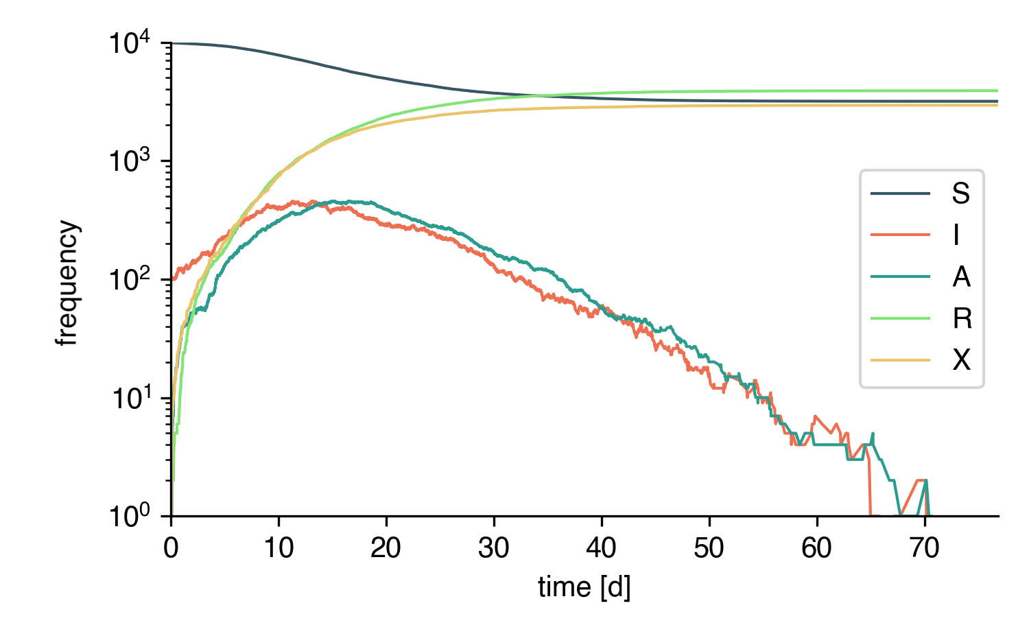
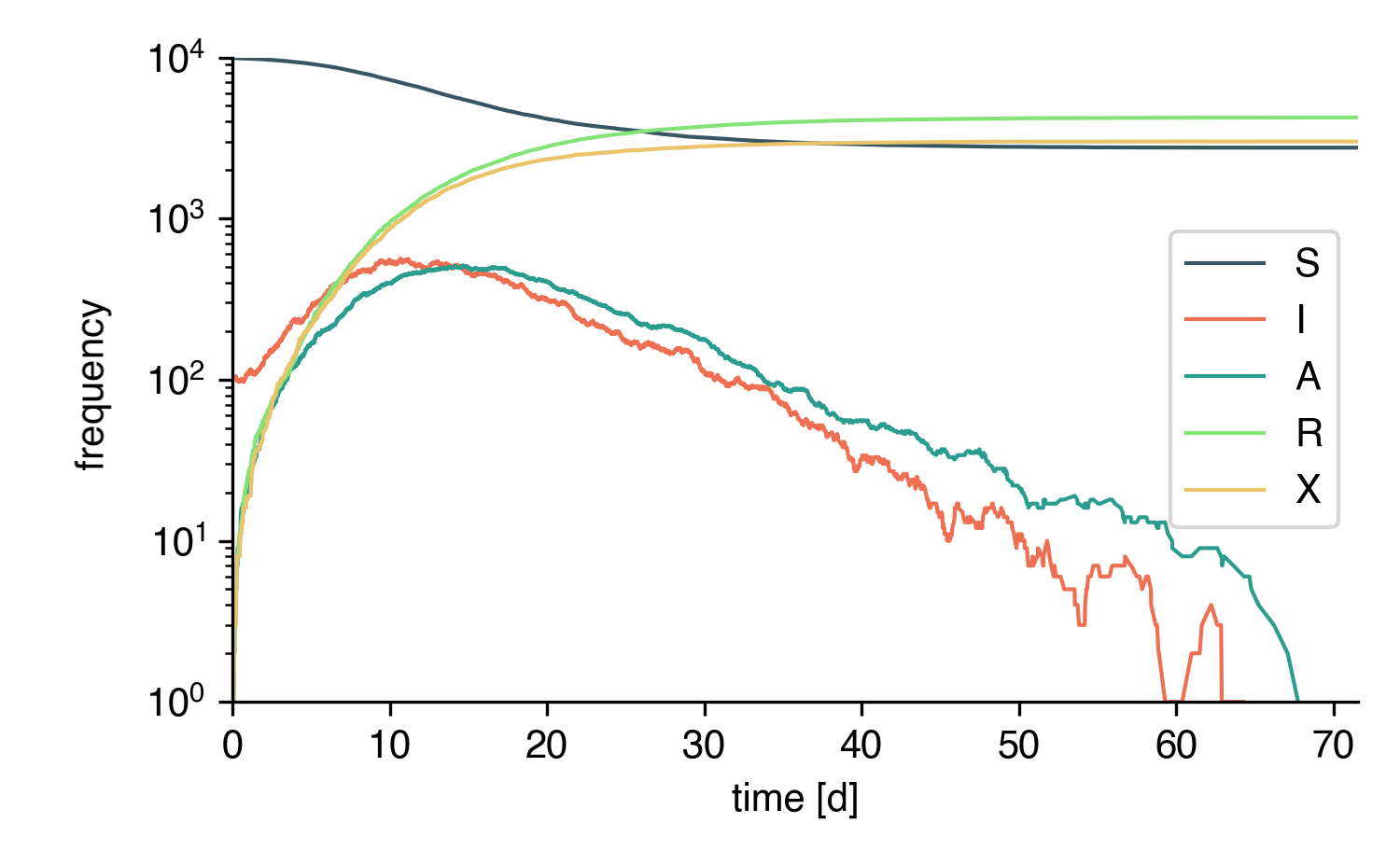
Well-Mixed Systems
In principle, EpiModel and SymbolicEpiModel both offer
similar comfortable frameworks to simulate well-mixed systems
stochastically with their simulate() method. Yet,
things like conditional transmission processes cannot
be simulated.
Using, StochasticEpiModel we can tell the model to assume well-mixed contact structure with mean contact number \(k_0\). This means that StochasticEpiModel will assume that every node has \(k_0\) neighbors at every time and when a node reacts in a (possibly conditional) link transmission, \(k_0\) neighbors are sampled from the remaining node set to represent this node's neighbors at the current moment. Then, one of those sampled neighbors is chosen for a reaction (for a conditional link transmission, all neighbors are iterated).
It's simple enough to adjust the model defined above to run on a well-mixed model. Simply re-define the model as well-mixed with
model.set_well_mixed(N, k0)
or initiate the model as a well-mixed model:
model = StochasticEpiModel(
           compartments=compartments,
           N=N,
           well_mixed_mean_contact_number=k0
           )
This is a simulation of the same model on a well-mixed system:
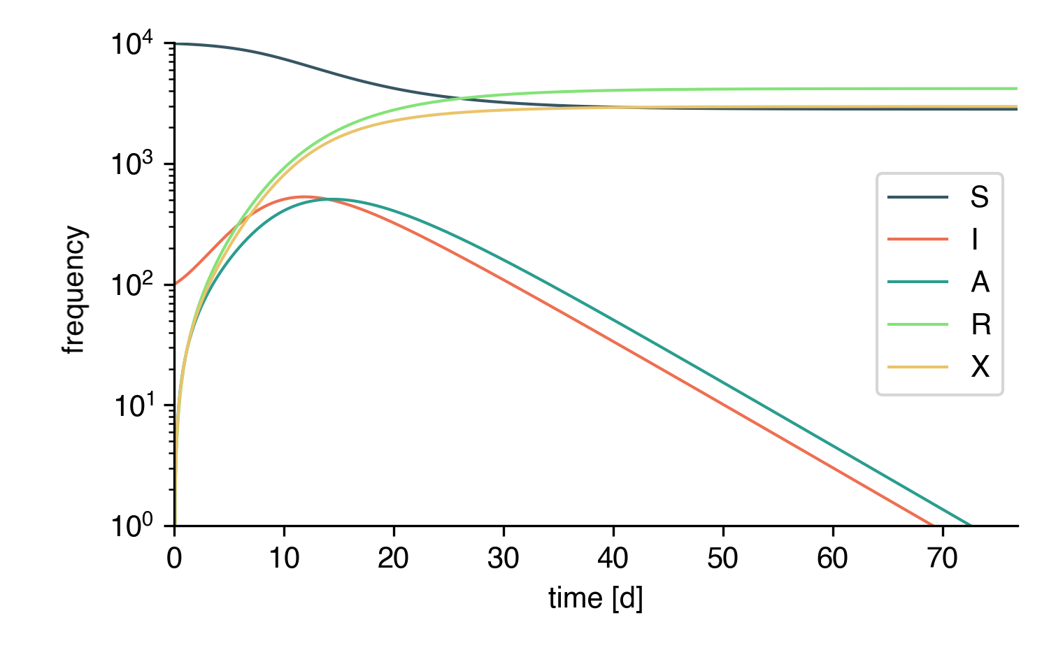
We can compare the whole thing to a deterministic implementation of a similar model. To this end, we adjust the conditional link transmission rate to be reformulated as a transmission process. The contact tracing mechanism can be approximated by the following reaction equation
that can be written as
The motivation here is as follows.
Symptomatic infectious individuals I are quarantined with rate \(\kappa\), i.e. \(\kappa\times I\) individuals are isolated per unit time. A focal I individual has contact to \(k_0\times I/N\) of such infecteds on average and on average, it's going to be traced by a fraction \(p\) of those contacts. In total, the tracing rate is therefore equal to \(\kappa p k_0 I/N\) (Note that the mathematically more rigorous derivation is a bit more tedious).
Hence, we define the equivalent deterministic model as
link_transmission = [
    ('I', 'S', k0*infection_rate*0.7, 'I', 'I'),
    ('I', 'S', k0*infection_rate*0.3, 'I', 'A'),
    ('A', 'S', k0*0.5*infection_rate*0.7, 'A', 'I'),
    ('A', 'S', k0*0.5*infection_rate*0.3, 'A', 'A'),
    ('I', 'I', quarantine_rate*k0*p, 'I', 'X'),
]

model = EpiModel(
           compartments=compartments,
           initial_population_size=N,
           )\
       .set_processes(node_transition + link_transmission)\
       .set_initial_conditions({
                                   'S': N-100,
                                   'I': 100
                               })
t = np.linspace(0,100,1000)
result = model.integrate(t)
while keeping everything else as it is.
And this is the result: