Symbolic Models
Symbolic models are more powerful than pure numeric models. In fact, they can do everything that an EpiModel can do and more. Symbolic models are named like that because they are based on sympy symbols (and as such function as a hybrid between numeric evaluations and computer algebra systems).
Example: SIRS model
First, we define all compartments and parameters as sympy symbols
from epipack import SymbolicEpiModel
import sympy as sy

S, I, R, eta, rho, omega = sy.symbols("S I R eta rho omega")
With these symbols, we can set up the base model
SIRS = SymbolicEpiModel([S,I,R])\
    .set_processes([
        (S, I, eta, I, I),
        (I, rho, R),
        (R, omega, S),
    ])
That's all. Now we can analyze the system analytically.
ODEs
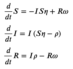
Let's begin by looking at the ODEs of the deterministic model.
In [79]: SIRS.ODEs()
Out[79]:
[Eq(Derivative(S, t), -I*S*eta + R*omega),
 Eq(Derivative(I, t), I*(S*eta - rho)),
 Eq(Derivative(R, t), I*rho - R*omega)]
In a jupyter notebook, we can display the ODEs with LaTeX.
SIRS.ODEs_jupyter()
Fixed Points and Linear Stability
Usually, we're interested in fixed points of the system. You can let sympy find them.
SIRS.find_fixed_points()
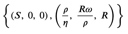
Also, we're interested in the linear stability of these fixed points. Let's use the fixed point
First, we need to eliminate the unset value \(R\) by using the normalization condition
The linear stability can now be found using the following method
>>> SIRS.get_eigenvalues_at_fixed_point({
...     S : rho / eta,
...     I : eta * omega / rho / (omega + rho),
...     R : eta / (omega + rho),
... })
{-omega*(eta**2 + omega*rho + rho**2)/(2*rho*(omega + rho)) - sqrt(omega*(eta**4*omega - 2*eta**2*omega**2*rho - 6*eta**2*omega*rho**2 - 4*eta**2*rho**3 + omega**3*rho**2 + 2*omega**2*rho**3 + omega*rho**4))/(2*rho*(omega + rho)): 1,
 -omega*(eta**2 + omega*rho + rho**2)/(2*rho*(omega + rho)) + sqrt(omega*(eta**4*omega - 2*eta**2*omega**2*rho - 6*eta**2*omega*rho**2 - 4*eta**2*rho**3 + omega**3*rho**2 + 2*omega**2*rho**3 + omega*rho**4))/(2*rho*(omega + rho)): 1,
 0: 1}
The eigenvalues contain parts that can become complex - explaining the emergence of oscillations in this system.
Of course, the epidemic threshold is a central observable of interest. To find this threshold, we need to compute the linear stability at the disease free state \(Y = (1,0,0)\).
>>> SIRS.get_eigenvalues_at_disease_free_state()
{-omega: 1, eta - rho: 1, 0: 1}
The disease free state therefore becomes unstable when \(\eta > \rho\), i.e the epidemic threshold is given as
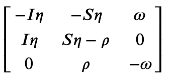
Jacobian
In order to analyze linear stability, we need access to the system's Jacobian that can be found as
>>> SIRS.jacobian()
Analyze Numerically and Stochastically
SymbolicEpiModel inherits all analysis methods from EpiModel. Hence, we can do everything that we can do with an EpiModel. All we need to do is to set numerical parameter values
SIRS.set_parameter_values({eta: 2.5, rho: 1.0, omega:1/14})
t = np.linspace(0,40,1000)
result = SIRS.integrate(t)
N = 10000
SIRS = SymbolicEpiModel([S,I,R],N)
t_sim, result_sim = SIRS.simulate(40)
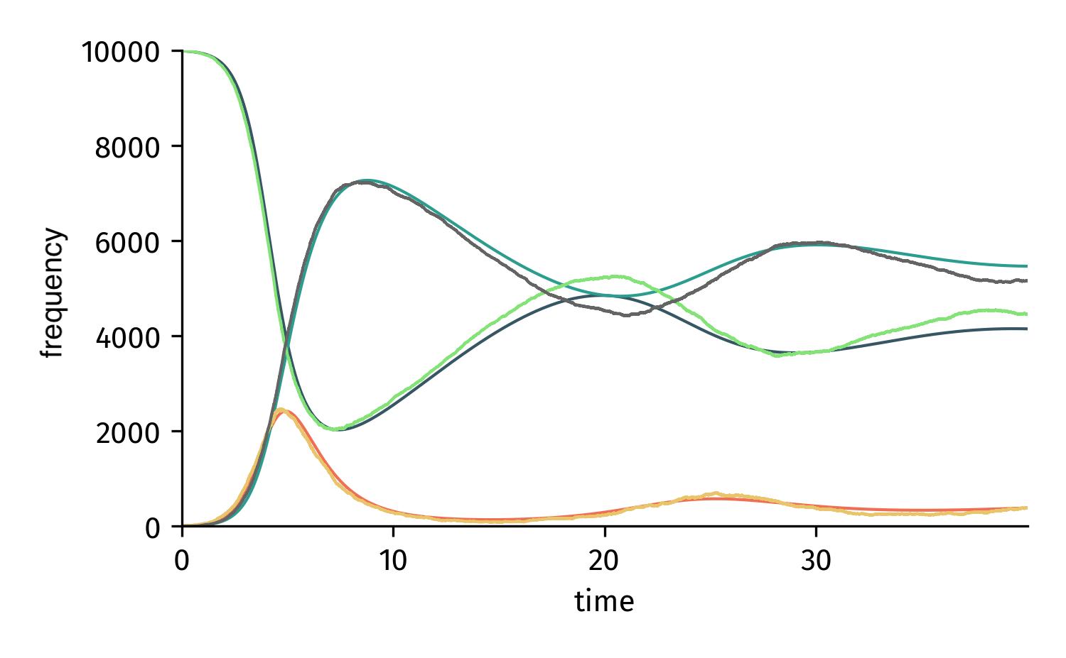
Integrated/simulated system based on a SymbolicEpiModel.
Interactive Analysis
In jupyter notebooks, a SymbolicEpiModel can be used with an interactive widget.
Make sure to first run
%matplotlib widget
Now we define the model as before, but as parameters we use the infectious period \(\tau\) (instead of the recovery rate \(\rho\)) and the basic reproduction number \(R_0 = \eta\tau\).
S, I, R, R0, tau, omega = sympy.symbols("S I R R_0 tau omega")

I0 = 0.01
model = SymbolicEpiModel([S,I,R])\
             .set_processes([
                    (S, I, R0/tau, I, I),
                    (I, 1/tau, R),
                    (R, omega, S),
                ])\
             .set_initial_conditions({S:1-I0, I:I0})
Now we set parameter
ranges instead of parameter values with
epipack.interactive.Range and
epipack.interactive.LogRange.
Each parameter value that's associated with a range will be rendered as a slider.
We can define these parameters like so:
from epipack.interactive import InteractiveIntegrator, Range, LogRange

parameters = {
    R0: LogRange(min=0.1,max=10,step_count=1000),
    tau: Range(min=0.1,max=10,value=8.0),
    omega: 1/14
}
And then we just run the integrator.
t = np.logspace(-3,2,1000)
InteractiveIntegrator(model, parameters, t, figsize=(4,4))
Pure ODE Models
In case you already have an ODE system ready to go,
you can define it with epipack.symbolic_epi_models.SymbolicODEModel
without going through the hassle of converting it
to reaction processes. Simply define the equations
as a list of sympy equation objects:
import sympy as sy
from epipack import SymbolicODEModel

S, I, R, alpha, beta, t = sy.symbols("S I R alpha beta t")

ODEs = [
    sy.Eq(sy.Derivative(S, t), -alpha*S*I),
    sy.Eq(sy.Derivative(I, t), +alpha*S*I - beta*I),
    sy.Eq(sy.Derivative(R, t), +beta*I),
]

model = SymbolicODEModel(ODEs)
epipack infers the compartments automatically. Note that stochastic simulations are not possible with this model since events cannot be inferred from ODEs.