Numeric Models
A Simple Example
Let's say we want to define a (S)usceptible, (E)xposed, (I)nfected, (R)ecovered system where symptomatic individuals are (Q)uarantined with a quarantine rate \(\kappa\).
The reaction equations read
i.e. symptomatic infecteds infect susceptibles upon contact with rate \(\alpha\), who become then exposed. Exposed individuals become symptomatically infected and infectious with rate \(\omega\), symptomatic infecteds recover with rate \(\beta\) or are discovered and quarantined with rate \(\kappa\).
The first thing we need to do is to set up a model with the right compartments
using the base class epipack.numeric_epi_models.EpiModel.
import epipack as epk

S, E, I, R, Q = list("SEIRQ")
model = epk.EpiModel(compartments=[S,E,I,R,Q])
Automatically, the model maps compartments to indices in a compartment vector \(Y=(S,E,I,R,Q)\). We can check that
>>> [ model.get_compartment_id(C) for C in [S, E, I, R, Q]]
[0, 1, 2, 3, 4]
We can also get a compartment by index.
>>> [ model.get_compartment(iC) for iC in range(5) ]
["S", "E", "I", "R", "Q"]
Now, let's define some rate values in units of 1 per days and set the reaction processes
infection_rate = 1/2
recovery_rate = 1/4
quarantine_rate = 1/6
symptomatic_rate = 1

model.set_processes([
    # S + I (alpha)-> E + I
    (S, I, infection_rate, E, I),

    # E (omega)-> I
    (E, symptomatic_rate, I),

    # I (beta)-> R
    (I, recovery_rate, R),

    # I (kappa)-> Q
    (I, quarantine_rate, Q),
])
Let's say that initially, we have 1% infecteds.
I0 = 0.01
model.set_initial_conditions({S: 1-I0, I: I0})
epipack assumes that all compartments that are not explicitly set are associated with an initial condition of \(Y_i = 0\).
Now, we can integrate the ODEs and plot the result
import numpy as np
import matplotlib.pyplot as plt

t = np.linspace(0,100,1000)
result = model.integrate(t)

plt.figure()
for compartment, incidence in result.items():
    plt.plot(t, incidence, label=compartment)

plt.xlabel('time [days]')
plt.ylabel('incidence')
plt.legend()
plt.show()
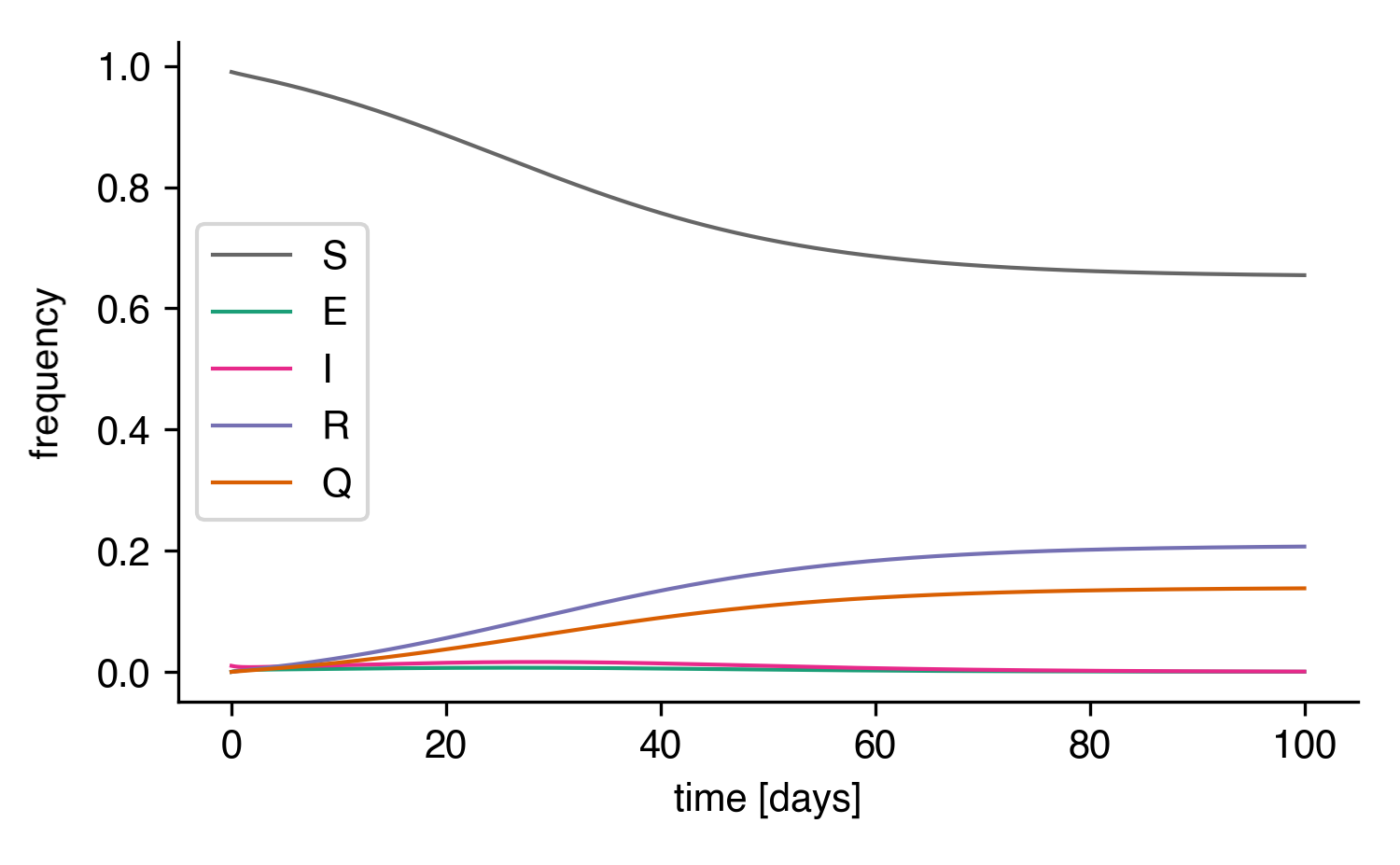
The integrated SEIRQ model.
Note that we do not have to use model.set_processes.
We can be more explicit by using
model.add_transition_processes()(processes \(Y_i\rightarrow Y_j\), \(\varnothing \rightarrow Y_j\), \(Y_i \rightarrow \varnothing\)),model.add_transmission_processes()(processes \(Y_i+Y_j\rightarrow Y_k+Y_\ell\)),model.add_fission_processes()(processes \(Y_i\rightarrow Y_j+Y_k\)),model.add_fusion_processes()(processes \(Y_i+Y_j\rightarrow Y_k\)),
Controlled Definition with Events
Setting up a model using reaction equations comes
with the comfort of not having to worry about symmetry
in the system. Yet, it also takes away control to some
extent. EpiModel is an event-based model which means
that internally, processes are saved as events that
take place with a rate and influence the system state
by de-/increasing integer compartment counts.
We can take back control by defining the events ourselves. An event is defined by a list of compartments that couple, a rate, and a list of compartment count changes. For coupled, i.e. quadratic terms, we define
model.set_quadratic_events([
    ( (S, I),
      infection_rate,
      [ (S, -1), (E, +1) ]
    ),
])
You should read that as follows: The set of all
quadratic events is given by a single infection event.
In that event, compartments S and I couple and react
with rate infection_rate. When such an event takes place,
the count of susceptibles S decreases by one and the
count of exposed increases by one.
We can define linear events in a similar manner
model.set_linear_events([
    # E (omega)-> I
    (  (E,),
       symptomatic_rate,
       [ (E, -1), (I, +1)],
    ),
    # I (beta)-> R
    (  (I,),
       recovery_rate,
       [ (I, -1), (R, +1)],
    ),
    # I (kappa)-> Q
    (  (I,),
       quarantine_rate,
       [ (I, -1), (Q, +1)],
    ),
])
A model that's defined in this way is in every way equal to the model defined above.
Stochastic Simulations
From how events are defined, stochastic simulations are straight-forward to set up: We use Gillespie's stochastic simulation algorithm (SSA) where all events are collected in an event set \(E\) and associated with rate \(\lambda_e\) (with \(e\in E\)). An event is also associated with a state change vector \(\Delta Y^{(e)}\), for instance \(\Delta Y^{(e)}=(-1,+1,0,0,0)\) for the event \(S+I\rightarrow E+I\). At each time point, a time leap \(\tau\) is sampled from
where \(\mathcal E(\Lambda)\) is an exponential distribution with mean \(\Lambda^{-1}\). Subsequently, an event \(e\) takes place with probability
by setting
We don't have to do much to simulate. We set up the model with an integer initial population size.
N = 1000
I0 = 100
model = epk.EpiModel([S,E,I,R,Q],initial_population_size=N)
model.set_processes([
    (S, I, infection_rate, E, I),
    (E, symptomatic_rate, I),
    (I, recovery_rate, R),
    (I, quarantine_rate, Q),
])
model.set_initial_conditions({S: N-I0, I: I0})
And simply simulate until \(t=100\mathrm{d}\).
t, result = model.simulate(100)
and plot the result
plt.figure()
for compartment, incidence in result.items():
    plt.plot(t, incidence, label=compartment)

plt.xlabel('time [days]')
plt.ylabel('incidence')
plt.legend()
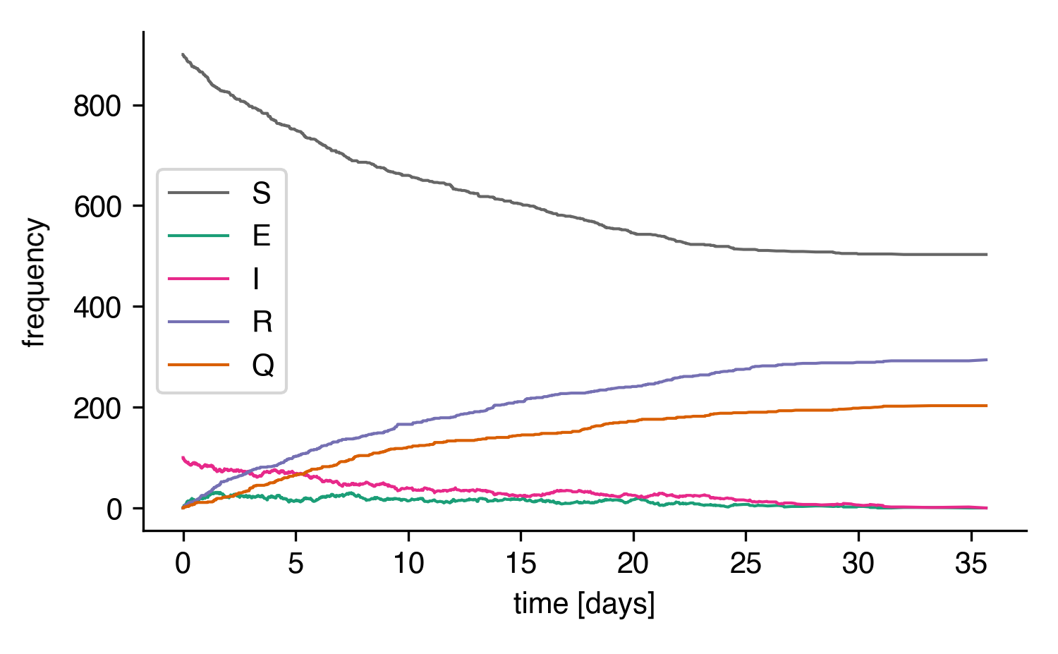
A stochastic simulation of the SEIRQ model.
Let's compare the whole thing to the result of the integrated ODEs:
tt = np.linspace(0,100,1000)
result_int = model.integrate(tt)

for compartment, incidence in result_int.items():
    plt.plot(tt, incidence)
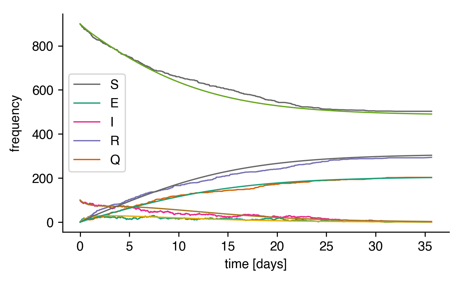
Stochastic simulation of the SEIRQ model compared to the integrated ODE system.
Dynamically Changing Population Size
Let's come back to the model defined in the introduction:
It's a modified SIR system where new susceptibles are born with constant rate \(\gamma\).
Let's set up an EpiModel.
import epipack as epk

N = 1000
S, I, R = list("SIR")
model = epk.EpiModel([S,I,R],
                     initial_population_size=N)

alpha = 1/2
beta = 1/4
gamma = 1
I0 = 100

model.set_processes([
        (S, I, alpha, I, I),
        (I, beta, R),
        (None, gamma, S),
    ])
Note that we're hit with the following warnings:
UserWarning: This model has processes with a fluctuating number of agents.
Consider correcting the rates dynamically with the attribute
correct_for_dynamical_population_size = True
UserWarning: events do not sum to zero for each column: 1.0
epipack noticed that the population size will not stay constant. If this is intended, reaction rates of quadratic couplings will have to be rescaled by the dynamically changed population size.
Tell the model to do this by setting
model.correct_for_dynamical_population_size = True
Ideally, you already knew that beforehand, which is why you want to initiate the model with this behavior:
model = epk.EpiModel([S,I,R],
                     initial_population_size=N,
                     correct_for_dynamical_population_size=True,
                     )
Now, we can integrate the ODEs and simulate the system
t, result_sim = model.simulate(4000)
result_int = model.integrate(t)
This is the initial development:
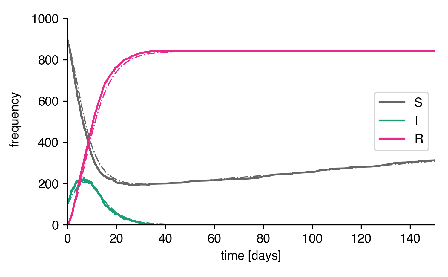
Stochastic simulation and ODE integration of the SIR-birth model.
As we can see, ODE solution and stochastic solution line up relatively well. How does it look for longer times though?
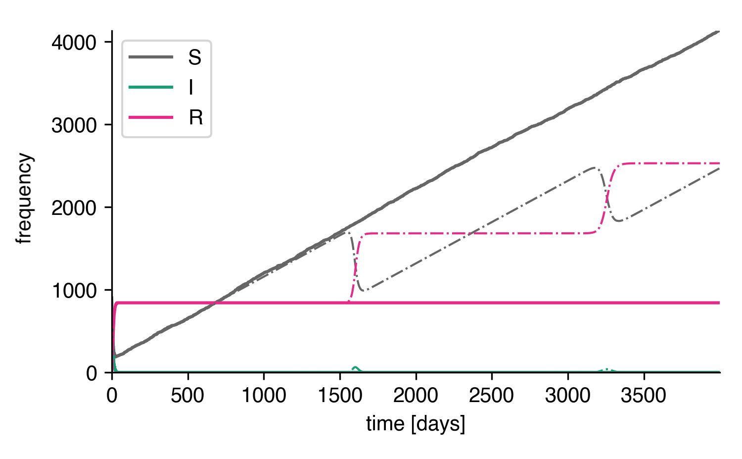
Longer times.
A new effect! Apparently, a second and a third wave rapidly depletes the grown susceptible population in the deterministic system. In order to understand what's going on, we can take a look at the curves on a log scale.
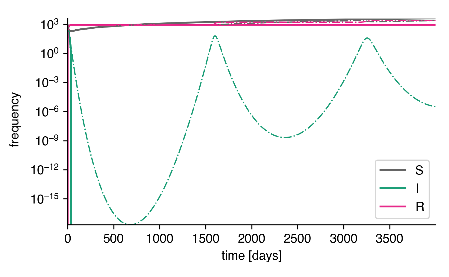
Longer times with log scale.
In the stochastic system, the number of infected individuals reaches \(I=1\) and is subsequently trapped in the absorbing state \(I=0\) with the next recovery event, while the deterministic system reaches incredibly low values of \(I\approx 10^{-15}\) until there are enough susceptible individuals such that another waves may occur. In reality, a value of \(I=10^{-15}\) would not be reached, even in very large systems. Such a low value just implies that the disease dies out eventually.
We can, however, assume that reimports of single infecteds can trigger second waves when there are enough susceptible individuals. Such a behavior may be mimicked by adding another birth process with a small rate and simulating again.
model.add_transition_processes([
        (None, 1e-3, I),
    ])
t, result_sim = model.simulate(4000)
As we can see, doing so reconciles the stochastic system with the deterministic system, at least qualitatively. The first peak is reproduced. The second peak is not reproduced because no reimport happened up to time \(t=4000\mathrm{d}\) in this particular simulation.
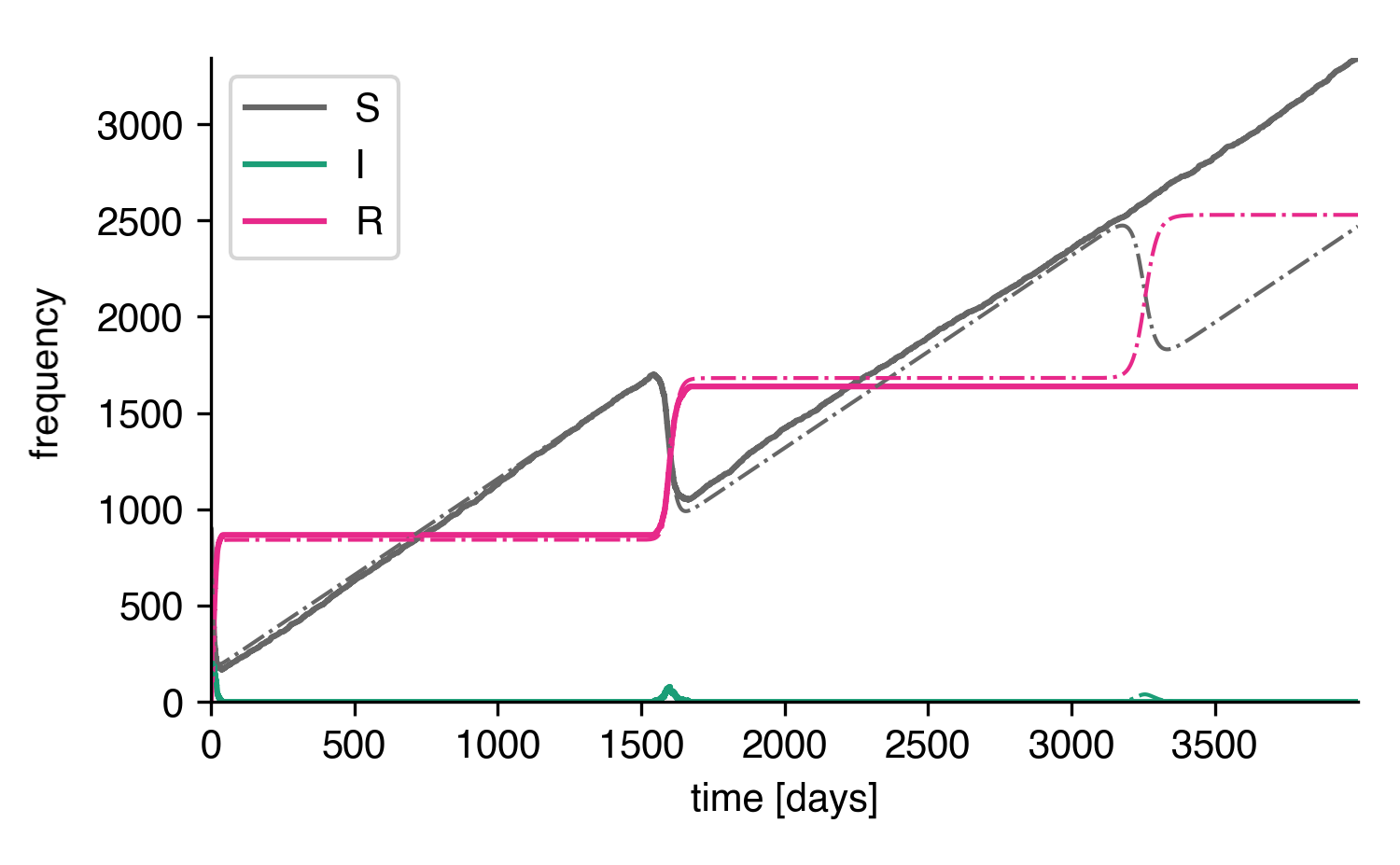
Stochastic system with reimports.
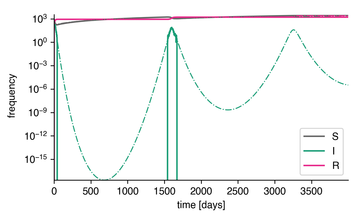
Stochastic system with reimports on a log scale.
Integrating Until a Condition is Reached
We can also specify conditions at which the integration of a model should be stopped.
from epipack import SIModel

model = SIModel(infection_rate=1.0)
model.set_initial_conditions({"S":0.9,"I":0.1})

thresh = 0.5
_S = model.get_compartment_id("S")

# stop integration when the frequency of
# susceptibles reaches 50%
stop_condition = lambda t, y: thresh - y[_S]

t0 = 0
t, res = model.integrate_until(t0,stop_condition)